Biases in Traditional Retention and Churn Analysis
Why a cohort's churn rate falls as it ages, and why a blended churn rate tells you so little.
By Joseph Brady · November 16, 2026
Has your churn rate ever improved for a whole year while nobody on the retention team did anything differently?
The retention slide at a portfolio review shows one blended monthly churn rate for the whole book, with a target under it. That number gets better in a slow sales year and worse in a great one, and because every account counts once, it’s set mostly by the accounts worth the least. That’s the case for retiring it as a target and reading churn by cohort instead, as a share of what each cohort started with, by tier.
So why does a churn rate improve on its own? Demographers spelled it out in 1979, and two marketing professors brought it to customer data in 2007.
Demographers saw it first, in death rates
In 1979 three demographers, James Vaupel, Kenneth Manton and Eric Stallard, published a paper in Demography on what differences in frailty do to mortality statistics. A life table reports the chance of dying at each age. The trouble is that people differ in how frail they are, and the frailest die first. So the older a group gets, the more it’s made up of people who were robust to begin with, and the group’s death rate climbs more slowly than any one person’s risk does.
Their paper spelled out what that does to the numbers. Life tables that ignore those differences “overestimate current life expectancy … while underestimating rates of individual aging.” The group keeps changing underneath the average, and the average can’t show it.
Fader and Hardie found it in customers
Peter Fader of Wharton and Bruce Hardie of London Business School brought the same idea to customers. In their 2007 paper, “How to Project Customer Retention,” they took survival data that Michael Berry and Gordon Linoff had published for two segments of a subscription business and tried to forecast the last five years from the first seven. In the segment called Regular, the share of the previous year’s customers still active climbed from 63% in the first year to about 94% by the twelfth.
The usual read of a line like that is that customers get more loyal the longer they stay. Fader and Hardie’s model assumes every customer has their own fixed chance of leaving, one that never changes. The standard regressions missed year-12 survival by as much as 92%, and their model came within 4%. The rising line didn’t need anyone to change. In the paper’s words, “the observed phenomenon of increasing retention rates is simply a sorting effect in a heterogeneous population.” The library’s explainer on Fader and Hardie has their retention curve and the full forecast race.
In a 2010 Marketing Science paper subtitled “The Perils of Ignoring Heterogeneity,” they showed what ignoring it costs. Value a customer base with a single retention rate and the method “yields a downward-biased estimate” of what the remaining customers are worth, because one rate ignores that the customers still on the books are the ones least likely to leave.
Simpson’s paradox is the same math
Statisticians had already described the general version. In 1951 E. H. Simpson wrote a short note on how tables of counts combine, and in 1975 Peter Bickel, Eugene Hammel and J. W. O’Connell found the trap in Berkeley’s graduate admissions. The totals looked biased against women. Department by department, the bias ran slightly the other way, in women’s favor, because women had applied in larger numbers to the departments that admitted a smaller share of everyone. The name “Simpson’s paradox” came later. The library’s explainer on Simpson’s paradox walks through the Berkeley numbers.
The mix sets the rate
Every book of accounts is a mix of customers who were always likely to leave and customers who were always likely to stay. The blended churn rate is an average across that mix, weighted by how many of each are on the books. The leavers go first, so as a cohort ages the mix shifts toward the stayers and the rate falls. Sign a big new cohort and the mix shifts back, and the rate jumps. Either way the rate moved because the mix moved, even though no customer behaved any differently and nobody on your team did anything new.
The math, with two groups of accounts
Take one illustrative cohort of 200 accounts. Half are a fast group that churns 10% a month, and half are a slow group that churns 1% a month. Neither group’s rate ever changes.
In the first month the fast group loses 10 accounts and the slow group loses 1, so the blended rate is 11 out of 200, or 5.5%.
By the end of month 12, 28 of the fast group are left and 89 of the slow group. The fast group still churns 10% a month and the slow group still churns 1%, but the book is now about three-quarters slow group, and the blended rate is down to about 3.3%. Nobody changed. The leavers left first.
Now sign a new cohort of 200 with the same mix, 100 of each, in month 13. That month the blended rate falls to about 1.2%, the best it has ever looked, because the 200 new accounts count in the base and none of them can leave until the month after. The book is back to about 40% fast group, and in month 14, when the new accounts’ first losses show up, the rate jumps to about 4.6%. Again, nobody changed.
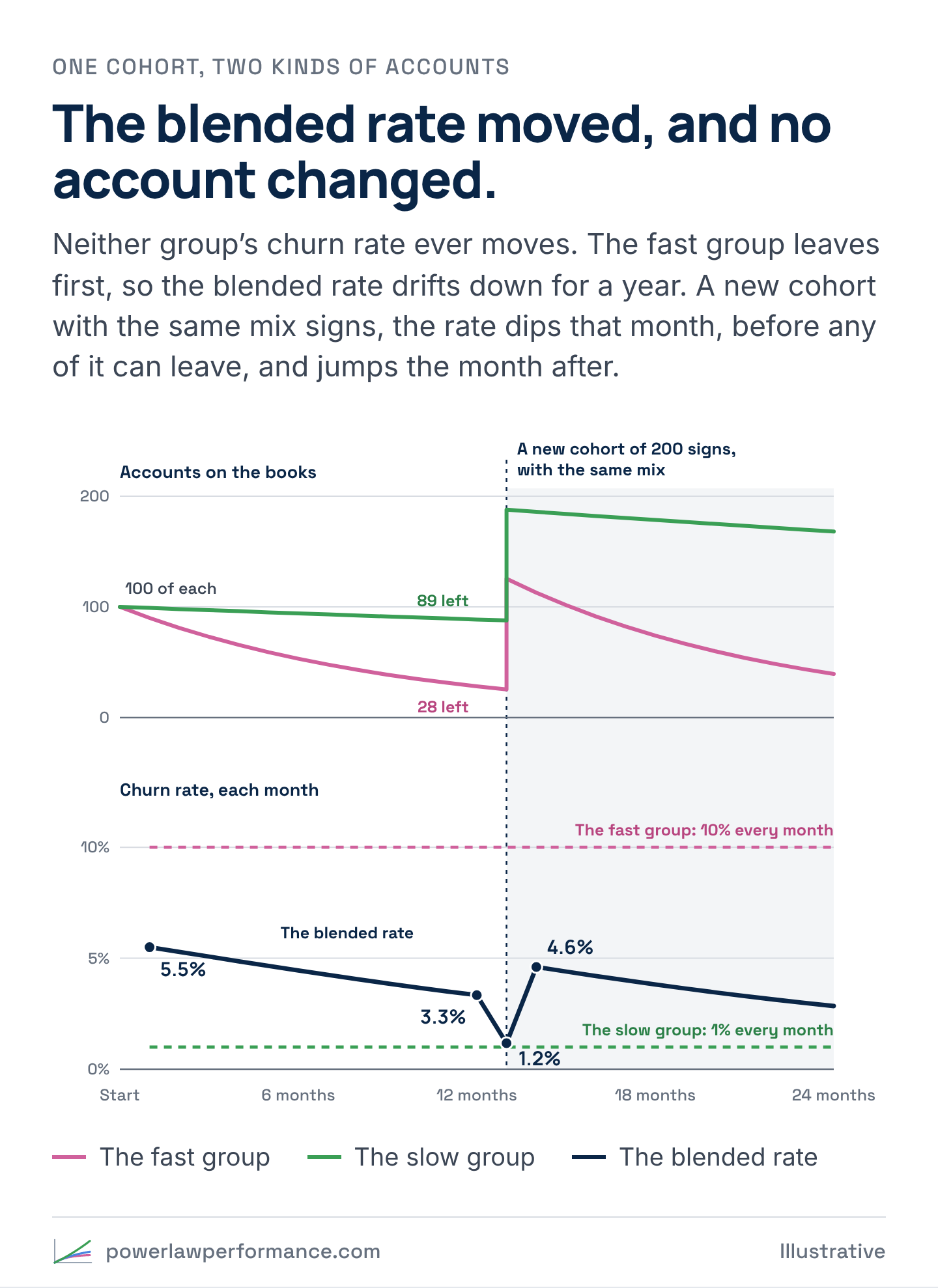
A review that reads only the blended line would have congratulated the retention team for a year, called month 13 its best month yet, and then asked what went wrong in month 14. The answer to both questions is the mix.
It gets stranger. Make the new accounts better than the old ones in both groups, churning 8% and 0.8% a month instead of 10% and 1%. Every group on the books is now as good as it was or better, and the blended rate still jumps, to about 3.9%. That’s Simpson’s paradox in a churn report. The total got worse and no group did.
How each rate is built
Most retention slides stop at the blended rate. The cohort view is built differently, and the difference is the whole point.
Take a book that starts in January and signs a new cohort every month (illustrative). Each cohort is the same two kinds of accounts as before, half churning 10% a month and half 1%. In July and August a promotion triples the volume, to 300 accounts a month, and 80% of them are the fast kind.
The blended rate stacks every cohort onto the book as it signs. Each month it takes every account lost that month, from every cohort, and divides by last month’s book plus the month’s new accounts, the base the losses come out of. The denominator compounds, because it carries every account that has signed and stayed.
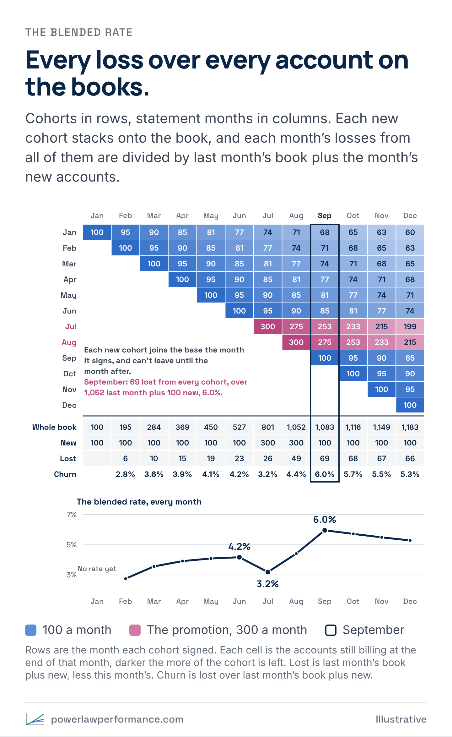
The rate climbs from 2.8% in February to 4.2% in June, mostly because each month’s brand-new cohort, which can’t leave yet, is a smaller share of a bigger base. In July, the month of the promotion, it drops to 3.2%: 300 new accounts swell the base, and none of them has had a month to leave. Then it jumps to 6.0% in September. Read on its own, the rate says the promotion improved retention in July and wrecked it by September. It can’t say why. More new accounts on the books and new accounts that leave faster both push it up the same way.
The cohort view counts each cohort against its own start. July’s losses are divided by July’s 300 and nobody else’s, so every cohort keeps its own rate. Then the cohorts are lined up at month zero, so they can be compared age for age.
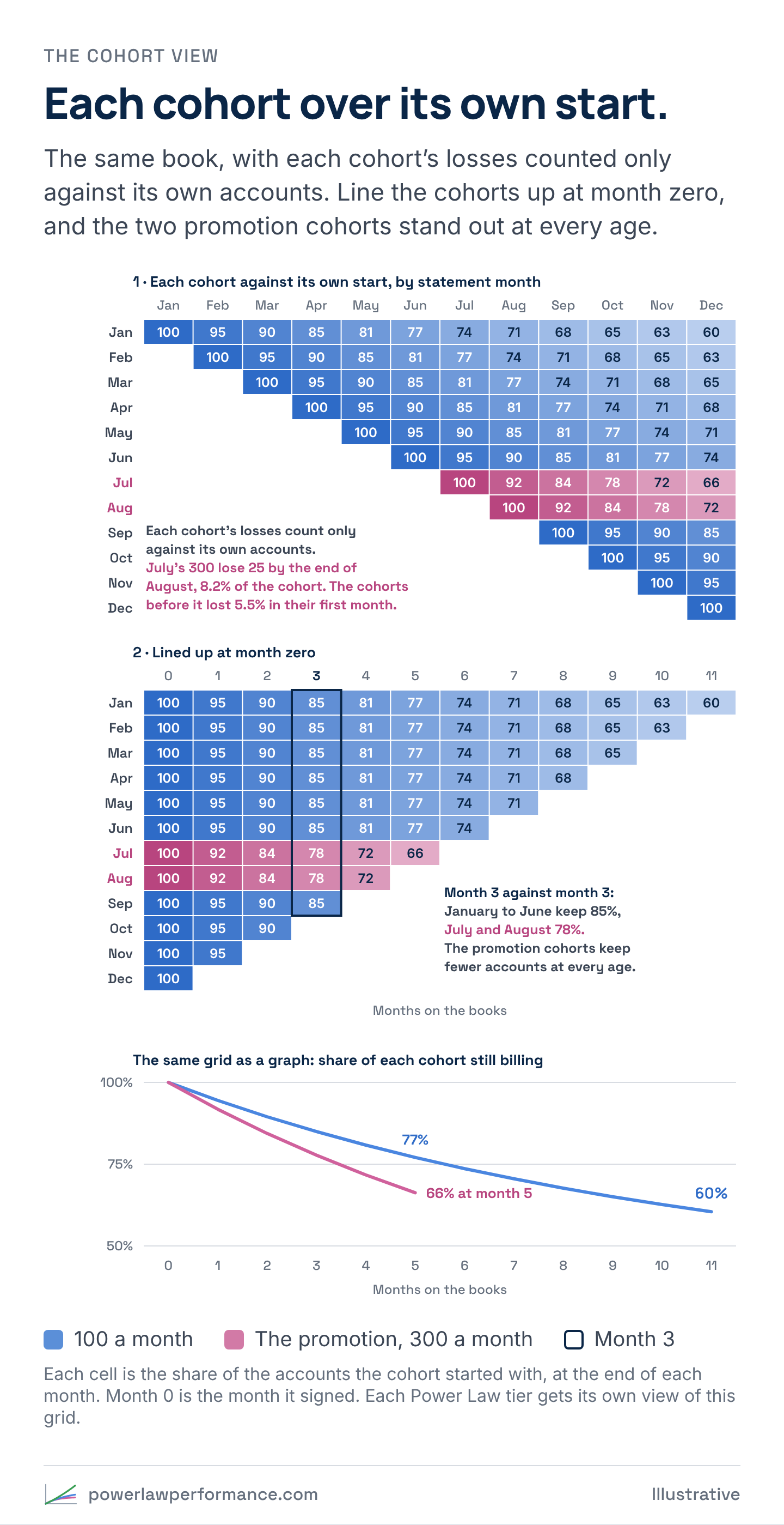
Read the lined-up grid month 3 against month 3. The January to June cohorts keep 85% of their accounts. July and August keep 78%. Those two cohorts really do leave faster, and the grid shows exactly which ones. If the fast leavers are your bottom tier, as they usually are, the same grid split by Power Law tier shows why: the promotion signed more bottom-tier accounts, and inside each tier nothing changed.
ABPRO_, the reporting platform Broad Eye Solutions builds, puts both views side by side, and each Power Law tier gets its own view of the cohort grid. Broad Eye Solutions clients review retention this way every month, cohort by cohort and tier by tier, in accounts and in revenue. If your team still reads one blended rate, book an ABPRO_ demo and see it on demo data.
What the research shows
Retention moves firm value more than margin or acquisition cost does. In Sunil Gupta, Donald Lehmann and Jennifer Ames Stuart’s 2004 study of five public firms, “Valuing Customers,” it moved value five times as much as margin did. The question that matters is whose retention.
Tenure isn’t value either. In “The Mismanagement of Customer Loyalty,” a 2002 Harvard Business Review study of four companies and more than 16,000 customers, Werner Reinartz and V. Kumar found that many long-tenure customers “barely generated a profit,” and many of the most profitable customers were short-term. A cohort that sorts down to its stayers hasn’t necessarily sorted down to its best accounts, which is why the tier split matters.
The customers at the highest risk of leaving aren’t automatically the right ones to chase. In “Retention Futility,” a 2018 paper built on two field experiments, Eva Ascarza found that picking who gets a save offer by risk of leaving worked worse than picking by how much the offer was predicted to move each customer. With the same campaign, targeting by predicted response cut churn by an extra 4.1 percentage points in the first study and 8.7 in the second. The library’s explainer on Ascarza covers both studies.
Reaching out can backfire. In a 2016 field experiment published in the Journal of Marketing Research, Ascarza, Raghuram Iyengar and Martin Schleicher tested proactive churn prevention by recommending plans to customers, and it raised churn. In the three months after the outreach, 10% of the treated customers left, against 6% of the control group.
What works is aiming at value and response together. In “Managing Churn to Maximize Profits,” a 2020 Marketing Science paper, Aurélie Lemmens and Sunil Gupta ranked customers by how much a retention campaign changed both their chance of leaving and their future cash flows, net of the campaign’s cost. In two field experiments, that approach produced significantly more profitable campaigns than the competing models.
Some customers do get stickier
The argument on the other side is that some customers really do get harder to lose the longer they stay, as your product becomes part of how they run their business. Sorting doesn’t rule that out. Fader and Hardie’s model assumes each customer’s chance of leaving is fixed, and it fits the data well. A good fit shows that sorting alone is enough to produce a rising curve. It doesn’t show that nobody changed.
From the totals alone, you can’t separate the two. A cohort that’s sorting and a cohort whose customers are getting stickier draw the same rising line on the retention slide.
Per-customer data can separate them, because you can follow the same accounts over time. If the accounts that stayed already looked different in their first month, in size, activity or where they came from, that’s sorting at work. If the same accounts’ usage and volume keep growing the longer they stay, that’s a sign some of the rise is real.
The demographers’ own finding cuts the other way too. Their point was that the group numbers understated how fast individuals were aging. In a customer book, sorting can make a cohort look steady while the customers inside it are slowly getting less loyal, and only the per-customer view shows it.
What it means for your retention team
- Stop comparing this month’s blended rate with last month’s. It moves with the age and the mix of the book, so a slow sales quarter flatters it and a strong one punishes it. If it has to stay on the slide, put the share of accounts in their first six months next to it.
- When a rate moves, check the mix before you credit the work. Break the number out by tier and by cohort age. If every group held steady and the total moved, the mix moved.
- Use per-customer data to tell sorting from real change. Before a program takes credit for an improving cohort, check whether the accounts that stayed looked different in their first month.
Two other pieces build these numbers a new way. Forecasting Next Year, One Layer at a Time builds next year from every cohort and every tier, then back tests it against what billed. Increase Revenue by Increasing Your Churn Rate reads retention by tier and lets you decide where the retention effort goes.
For the math-curious
The blended churn rate in any month is a weighted average of each group’s rate:
blended rate = (n₁c₁ + n₂c₂) ÷ (n₁ + n₂)
Here n is the number of accounts in each group at the start of the month and c is each group’s monthly churn rate. With fixed rates, a group of N accounts has N(1 − c)ᵗ left after t months. In the example, the fast group starts month 12 with 100 × 0.9¹¹ = 31.4 accounts and the slow group with 100 × 0.99¹¹ = 89.5, so that month’s rate is (31.4 × 10% + 89.5 × 1%) ÷ 120.9 = 3.34%. By the end of the month, 28.2 and 88.6 are left. The new cohort signs in month 13, and its accounts can’t leave until the month after. A month later 25.4 and 87.8 of the original accounts are left and the new cohort adds 100 to each group, so month 14 starts with 125.4 and 187.8, and its rate is (125.4 × 10% + 187.8 × 1%) ÷ 313.2 = 4.60%.
Fader and Hardie’s shifted-beta-geometric model replaces the two groups with a whole spread. Each customer’s chance of leaving in any period is fixed, and across customers those chances follow a beta distribution with two parameters, α and β. The cohort’s retention rate in period t works out to (β + t − 1) ÷ (α + β + t − 1), which rises every period even though no customer’s chance ever moves. The model fits in a spreadsheet, and the rising curve comes entirely from the mix.
Sources
- James W. Vaupel, Kenneth G. Manton and Eric Stallard, “The Impact of Heterogeneity in Individual Frailty on the Dynamics of Mortality,” Demography 16, no. 3 (1979): 439–454. doi:10.2307/2061224
- Peter S. Fader and Bruce G. S. Hardie, “How to Project Customer Retention,” Journal of Interactive Marketing 21, no. 1 (2007): 76–90. doi:10.1002/dir.20074 · authors’ copy
- Peter S. Fader and Bruce G. S. Hardie, “Customer-Base Valuation in a Contractual Setting: The Perils of Ignoring Heterogeneity,” Marketing Science 29, no. 1 (2010): 85–93. doi:10.1287/mksc.1080.0482
- E. H. Simpson, “The Interpretation of Interaction in Contingency Tables,” Journal of the Royal Statistical Society, Series B 13, no. 2 (1951): 238–241. doi:10.1111/j.2517-6161.1951.tb00088.x
- P. J. Bickel, E. A. Hammel and J. W. O’Connell, “Sex Bias in Graduate Admissions: Data from Berkeley,” Science 187, no. 4175 (1975): 398–404. doi:10.1126/science.187.4175.398
- Sunil Gupta, Donald R. Lehmann and Jennifer Ames Stuart, “Valuing Customers,” Journal of Marketing Research 41, no. 1 (2004): 7–18. doi:10.1509/jmkr.41.1.7.25084
- Werner Reinartz and V. Kumar, “The Mismanagement of Customer Loyalty,” Harvard Business Review 80, no. 7 (2002): 86–94. hbr.org
- Eva Ascarza, “Retention Futility: Targeting High-Risk Customers Might Be Ineffective,” Journal of Marketing Research 55, no. 1 (2018): 80–98. doi:10.1509/jmr.16.0163
- Eva Ascarza, Raghuram Iyengar and Martin Schleicher, “The Perils of Proactive Churn Prevention Using Plan Recommendations: Evidence from a Field Experiment,” Journal of Marketing Research 53, no. 1 (2016): 46–60. doi:10.1509/jmr.13.0483
- Aurélie Lemmens and Sunil Gupta, “Managing Churn to Maximize Profits,” Marketing Science 39, no. 5 (2020): 956–973. doi:10.1287/mksc.2020.1229