Is Your Business a Power Law Business?

A dealership tests its ads the way any good marketer would, and every challenger wins. Cars sold go up, the cost per car sold hits a record low, and years later the service revenue those sales were supposed to bring never shows up. The Free Lamborghini turns on one claim. A minority of buyers carries most of the long-term revenue, so a report that counts every sale the same steers the budget toward the buyers worth the least.

Is that true of your book? You can find out in an afternoon with a list of accounts, what each one brought in over the last year, and two averages.

What Pareto saw in the tax records

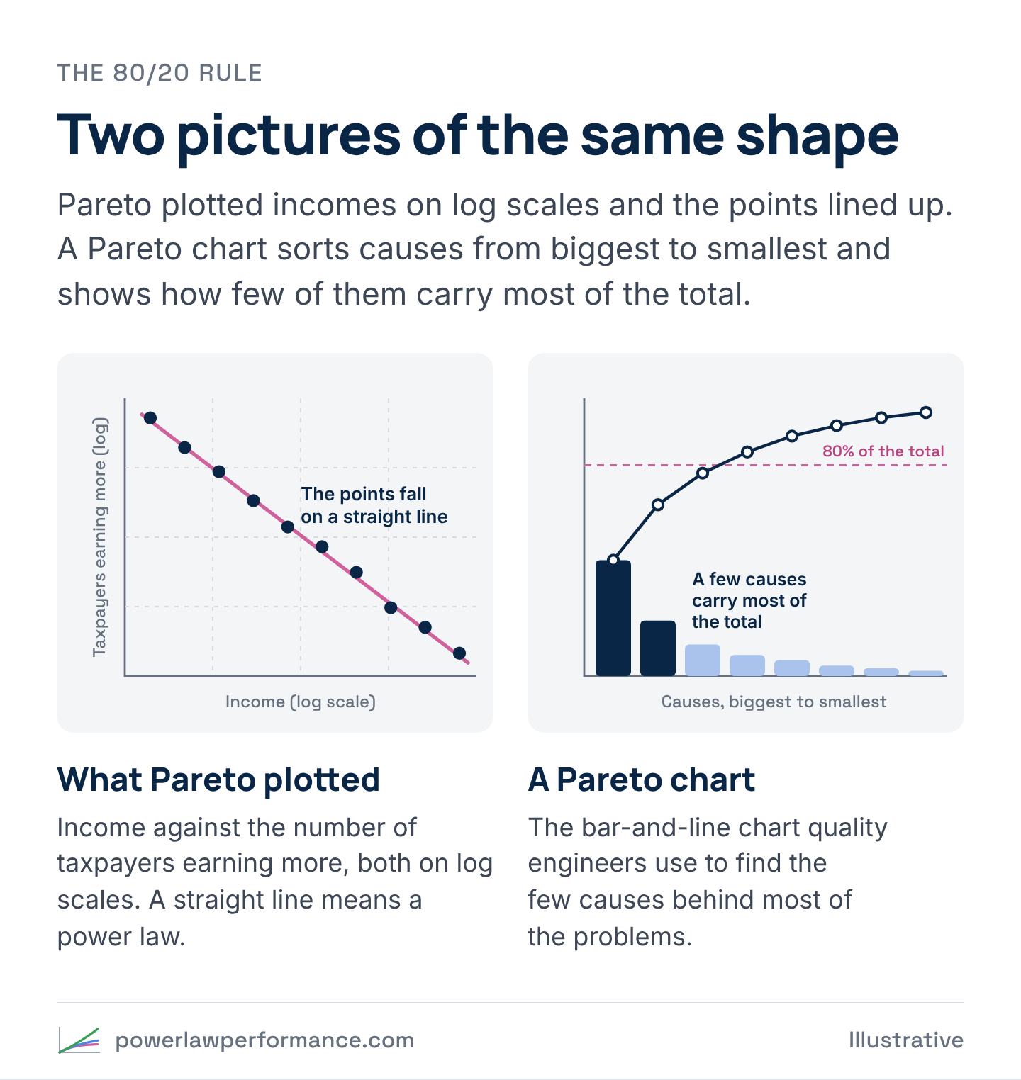
In the 1890s Vilfredo Pareto, an engineer turned economist teaching at Lausanne, wasn’t looking at customers at all. He wanted to know how income was spread across a population, so he gathered income-tax records from England, Ireland, Prussia, Saxony, Basel, Augsburg, several Italian cities and Peru. For each one he plotted an income level against the number of taxpayers earning more than it, with both axes on a log scale.

The points fell on a straight line. Every time the income level doubled, the number of people earning more dropped by the same fraction, and the lines from different countries and centuries had similar slopes, from 1.13 to 1.89 in his table. Pareto published it in his Cours d’économie politique in 1896–97, and he wouldn’t accept that it was chance.

The rule most people know came from Joseph Juran, a quality engineer. In the late 1930s, at General Motors, he was shown that the company’s executive pay fit one of Pareto’s models, and he started seeing the same shape in manufacturing defects, where a few causes produced most of the problems. In his 1951 Quality-Control Handbook he called it the Pareto principle, and “the vital few” followed in a 1954 paper. By 1975 he’d written a correction for Quality Progress, “The Non-Pareto Principle; Mea Culpa,” admitting, “I had mistakenly applied the wrong name to the principle.”

Pareto found a shape in incomes. Juran turned it into a universal rule, and “80/20” is the nickname it picked up along the way. The ratio was never part of the finding, as the Pareto and Juran explainer shows.

When you count profit instead of revenue

Robert Kaplan, the Harvard accounting professor who developed activity-based costing with Robin Cooper, took the shape somewhere more uncomfortable. He worked out what it costs to serve each customer, the orders, deliveries, support calls and custom terms as well as the product. Rank customers from most to least profitable, keep a running total, and the line climbs well past 100% of the company’s profit before it falls back, because the customers at the bottom lose money. That’s the whale curve.

Where the average account sits

In a bell-curve business, most accounts sit near the average, so the average account looks like a typical one. In a heavy-tailed business, a few big accounts pull the average up past almost everyone. Most accounts sit below it, a few sit far above it, and almost none sit at it. You don’t have an average business. You have a power law business, and every target set on the average account is set on an account your book barely has.

The two splits, on an illustrative book

The first move in the Free Lamborghini, check the shape, takes two averages. Take every account and what it brought in over the last twelve months. Split the book at the average. The accounts above it are above average, and the rest are below average. Then split each side at its own average. Above-average accounts that beat their group’s average are A, and the rest are B. Below-average accounts that beat their group’s average are C, and the rest are D. The method’s formal name is Power Law Nested Means, and the four groups it makes are Tiers A to D. A and B are above average. C and D are below average.

The chart runs the test on an illustrative book of 800 invented accounts drawn from a heavy-tailed curve. In that illustrative book, 23% of the accounts land above the average, and they bring in 76% of the revenue. Tier A alone is 5% of the accounts and 45% of the revenue. Tier D is 46% of the accounts and 6% of the revenue. The median account brings in just over a third of what the average account does, and only 38 of the 800 sit within 10% of the average either way.

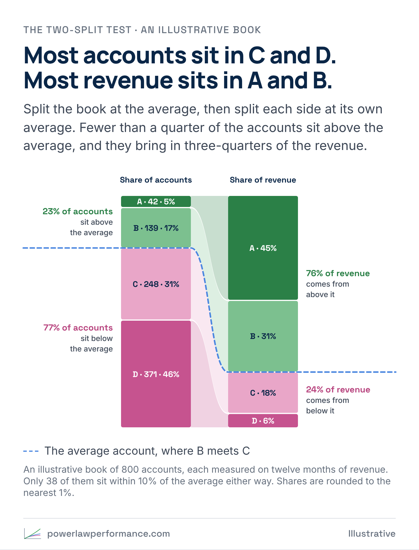
Compare that with a bell-curve book. Illustratively, in a bell curve whose spread is 30% of its average, half the accounts sit above the average and bring in about 62% of the revenue, and about a quarter of all the accounts sit within 10% of the average. In that book the average account means something. In the first one it describes almost nobody.

How to run it on your own book

All of this fits in a spreadsheet. You need one row per account and its revenue, month by month, for at least the last twelve months.

1. Pick the window. Twelve months or more, never one month. Add up what each account brought in. If a lot of your accounts joined partway through, use each account’s average month while it was active, so a new account doesn’t land in D just for being new.
2. Make the first split. Average the whole book, total revenue divided by the number of accounts. Accounts above that number are above average, and the rest are below average. Don’t expect two groups of the same size. How lopsided they come out is half the answer.
3. Make the second split. Average the above-average accounts on their own. The ones above that number are A, and the rest are B. Do the same with the below-average accounts. The ones above their average are C, and the rest are D.
4. Count both ways. For each tier, count the accounts and add up the revenue, then turn both into a share of the total and put them side by side.
5. Read it. If A and B are a small share of the accounts and carry most of the revenue, you’re in a power law, and every KPI that counts accounts (cost per lead, CAC, approval rate, churn rate) is weighted toward C and D, because that’s where the accounts are. If the two sides come out close to even, your book is closer to a bell curve.
6. Run it by channel. Keep the whole book’s cut points and count each channel’s accounts by tier, then do the same by campaign, source and rep. A channel that brings in plenty of accounts and almost no A’s is your free Lamborghini.
7. Keep the rule. Re-run it every month on a rolling twelve months, on the same rule, and watch accounts move between tiers.

Start with revenue, the number everyone already trusts. If you can get gross profit per account, run it on that too, and expect the shape to get sharper.

What the research shows

Even groceries show it. In a 2017 study of six years of Nielsen panel data covering more than 100,000 households, Byung-Do Kim, Vishal Singh and Russell Winer found a mean brand-level Pareto ratio of 0.73 across frequently purchased packaged goods. On average, the heaviest fifth of a brand’s buyers bought 73% of its volume, more for niche brands and less for big ones.

People show it too. In 2012 Ernest O’Boyle and Herman Aguinis tested 198 samples covering 633,263 researchers, entertainers, politicians and athletes, and a power law fit performance better than a bell curve in 186 of them. The same two splits work on a sales team, run on the value of what each rep closed, and the best and the rest explainer covers what that means for quotas and routing.

And profit shows it hardest. In a statement on customer profitability that cites Kaplan and V. G. Narayanan’s 2001 paper, the Institute of Management Accountants wrote, “Typically, about 20% of customers generate anywhere from 150% to 300% of company profits.” By the IMA’s account, the least profitable tenth can destroy anywhere from 50% to 200%. In revenue, D is small. In profit, part of D is negative.

Where the research pushes back

Does 80/20 hold everywhere? No. Byron Sharp, Jenni Romaniuk and Cathy Graham of the Ehrenberg-Bass Institute call their finding “Marketing’s 60/20 Pareto Law.” In packaged goods, they wrote in 2019, “A brand’s heaviest 20% of buyers generally contribute not much more than half of a brand’s sales,” 59% on average, from 68% for dog food down to 44% for hair conditioner. Their study and the Nielsen study measure concentration differently, and both come in under 80/20. Concentration varies by industry, so nobody else’s ratio tells you yours. A book that comes out flat isn’t a failed test. It’s the answer, and in a flatter book a KPI that counts accounts does less damage.

Time is the second pushback. In 1993 David Schmittlein, Lee Cooper and Donald Morrison showed that concentration figures are easy to compute and hard to interpret, and modelled the true level of concentration against what any one window shows. The same book measured over one month and over a year can give very different answers, which is why the test runs on twelve months or more.

The third is about the words “power law.” In 2009 Aaron Clauset, Cosma Rohilla Shalizi and M. E. J. Newman showed that the usual method, a straight line fitted on a log-log chart, “can produce substantially inaccurate estimates.” Tested properly, a power law held up in some of their 24 data sets and was ruled out in others. The two-split test doesn’t prove a power law either. It shows a heavy tail, a minority of accounts making up a majority of the results, and that’s all the business point needs.

And the numbers move. In Statistical Consequences of Fat Tails (2020), Nassim Nicholas Taleb shows that when the tail is heavy, the average of the accounts you have is a poor guide to the true average, and top-share figures computed the usual way come out wrong. One new whale moves your average and every cut point with it, so read the test for the shape, not the second decimal place.

What it means for your team

• Run it before the next target is set. The dealership’s cost-per targets inherited the average sale, and a minority of buyers carried that average. If your book splits like the chart, your cost per lead, CAC and quota are built on an account your book barely has.
• Make A to D the shared language. Marketing, sales, finance and customer success read the same four tiers, cut on the same rule, every month.
• Read every count-based KPI by tier. A churn rate, an approval rate or a cost per lead is mostly a C-and-D number, because that’s where the accounts are.
• Find your free Lamborghini. The source with the most accounts and the fewest A’s is the one every volume report tells you to scale.
• Then trace the A’s back. Once you know which accounts carry the book, ask what they looked like before anyone knew. That’s where signals come in.

For the math-curious

Pareto’s straight line has a formula. In a Pareto distribution, if x is an account’s value and xₘ is the smallest value, the share of accounts worth more than x is

P(X > x) = (xₘ / x)^α

The α is the steepness of Pareto’s log-log line, so his 1.13 to 1.89 are values of α. In that distribution, the top fraction p of accounts holds p^(1 − 1/α) of the total. Set p to 0.2, ask for 80%, and you get α ≈ 1.16. That’s all “80/20” is, one value of α. Smaller α means more concentration. At α = 2 the top fifth holds about 45%, and as α falls toward 1 its share climbs toward all of it.

Illustratively, at α = 1.16 about one account in ten sits above the average, and that tenth holds close to three-quarters of the total. Below α = 2 the variance is infinite, so a sample average keeps jumping as new whales arrive, which is the math behind Taleb’s warning. M. E. J. Newman’s 2005 review, “Power Laws, Pareto Distributions and Zipf’s Law,” is the standard primer.

---

Sources

1. Vilfredo Pareto, Cours d’économie politique, 2 vols. (Lausanne: F. Rouge, 1896–97). Catalogue record
2. J. M. Juran (ed.), Quality-Control Handbook (New York: McGraw-Hill, 1951); J. M. Juran, “The Non-Pareto Principle; Mea Culpa,” Quality Progress 8, no. 5 (1975): 8–9. Quoted from the Juran Institute reprint, p. 1. Juran Institute reprint
3. Robert S. Kaplan and V. G. Narayanan, “Measuring and Managing Customer Profitability,” Journal of Cost Management 15, no. 5 (2001): 5–15; Robert S. Kaplan and Robin Cooper, Cost & Effect (Boston: Harvard Business School Press, 1998). The quoted figures are from the Institute of Management Accountants, Statement on Management Accounting: Customer Profitability Management (2010), p. 2, which cites Kaplan and Narayanan.
4. Byung-Do Kim, Vishal Singh and Russell S. Winer, “The Pareto Rule for Frequently Purchased Packaged Goods: An Empirical Generalization,” Marketing Letters 28, no. 4 (2017): 491–507. doi:10.1007/s11002-017-9442-5
5. Ernest O’Boyle Jr. and Herman Aguinis, “The Best and the Rest: Revisiting the Norm of Normality of Individual Performance,” Personnel Psychology 65, no. 1 (2012): 79–119. doi:10.1111/j.1744-6570.2011.01239.x
6. Byron Sharp, Jenni Romaniuk and Cathy Graham, “Marketing’s 60/20 Pareto Law,” SSRN 3498097 (2019). doi:10.2139/ssrn.3498097
7. David C. Schmittlein, Lee G. Cooper and Donald G. Morrison, “Truth in Concentration in the Land of (80/20) Laws,” Marketing Science 12, no. 2 (1993): 167–183. doi:10.1287/mksc.12.2.167
8. Aaron Clauset, Cosma Rohilla Shalizi and M. E. J. Newman, “Power-Law Distributions in Empirical Data,” SIAM Review 51, no. 4 (2009): 661–703. doi:10.1137/070710111
9. Nassim Nicholas Taleb, Statistical Consequences of Fat Tails (STEM Academic Press, 2020). arXiv:2001.10488
10. M. E. J. Newman, “Power Laws, Pareto Distributions and Zipf’s Law,” Contemporary Physics 46, no. 5 (2005): 323–351. doi:10.1080/00107510500052444